Recently, our client called and said they had an emergency. They had to report to their Board of Directors in two days but could not make sense of 80,00 rows of sales data they had in Excel. They asked if we could help. As soon as we saw the data, we knew that Excel’s Pivot Table function provided the answer.
Many office professionals rely on Excel and know the basics very well, but Excel has many other features that can help save time and increase productivity. The problem is that we don’t know about them or, if we do, we do not know how to use them. One such feature is Pivot Tables. We would like to show you how to get started with Pivot Tables.
Needless to day, we took the data, built a Pivot Table and gave them their report in no time at all. They were thrilled and met their reporting deadline
Why Pivot Tables
It is one thing to summarize and analyze small amounts of data, but what happens when you have large amounts of data? This is where the Pivot Table feature comes into play. This tool helps you to organize and summarize selected columns and rows of data to create a desired report without changing the spreadsheet itself.
Steps to Create a Pivot Table
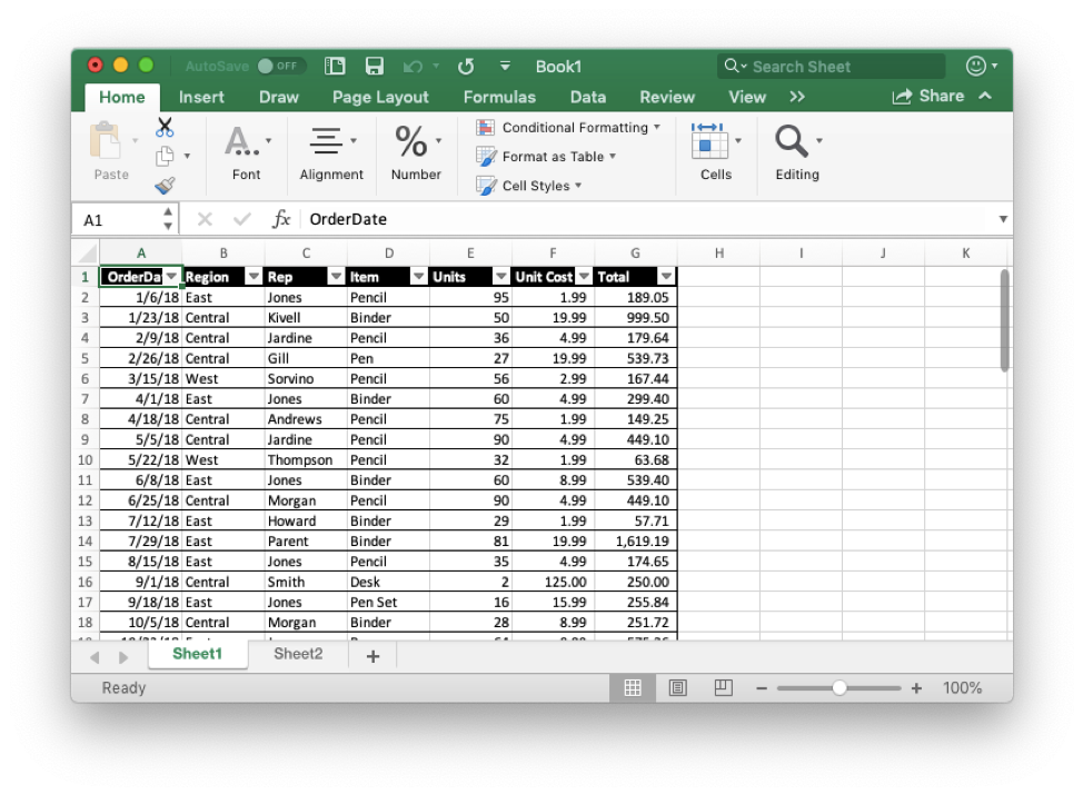
- Open your spreadsheet that you need to organize
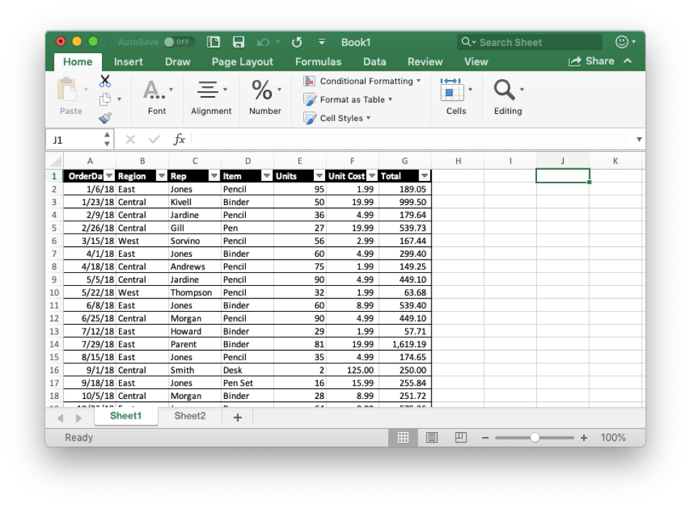
- Select the cell where you would like to create the Pivot Table, we will select J1
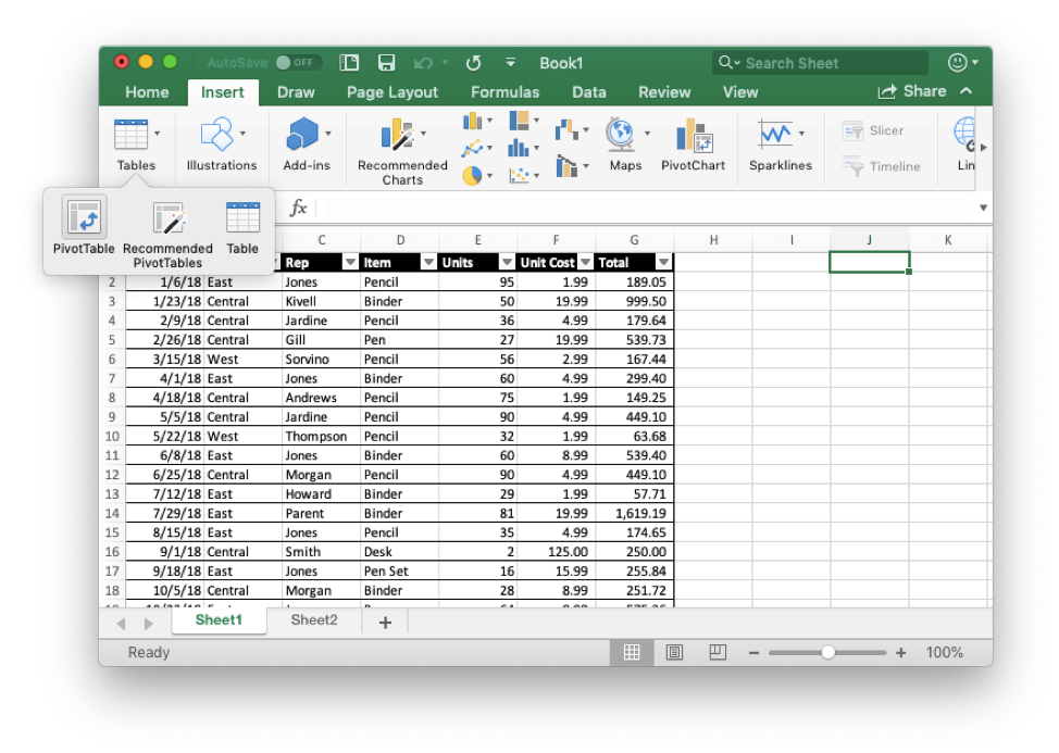
- Select the Insert tab from the toolbar and in the Tables group, click on Pivot Table.
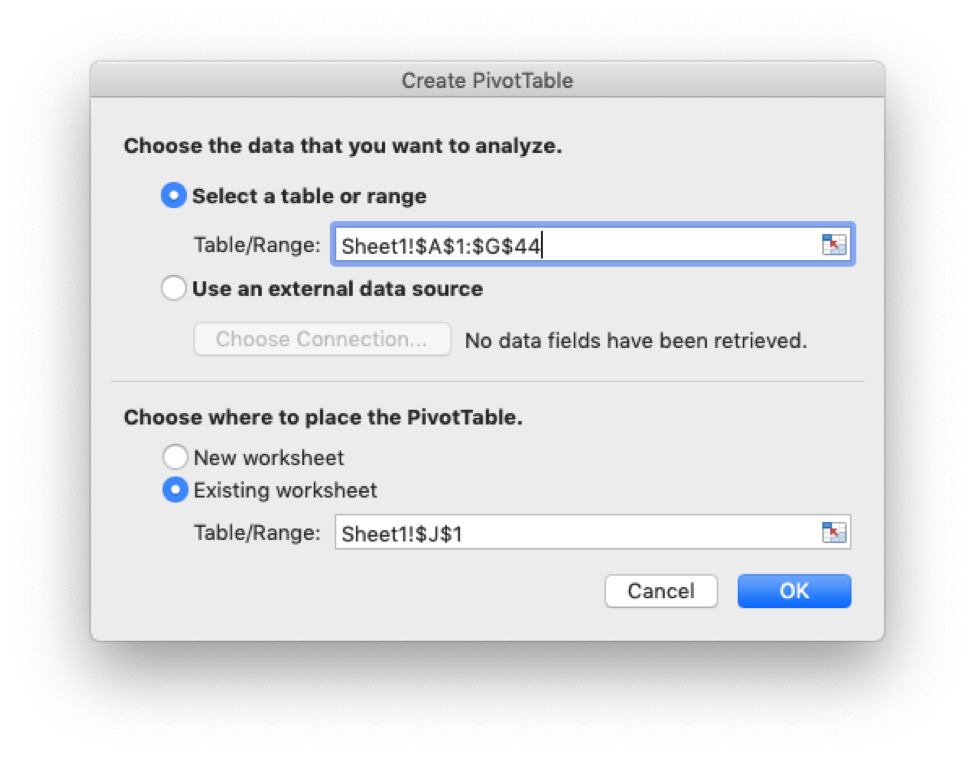
- When the Create PivotTable window appears, select the range of data and click OK. We selected A1 to G44.
You should see the following after you click OK: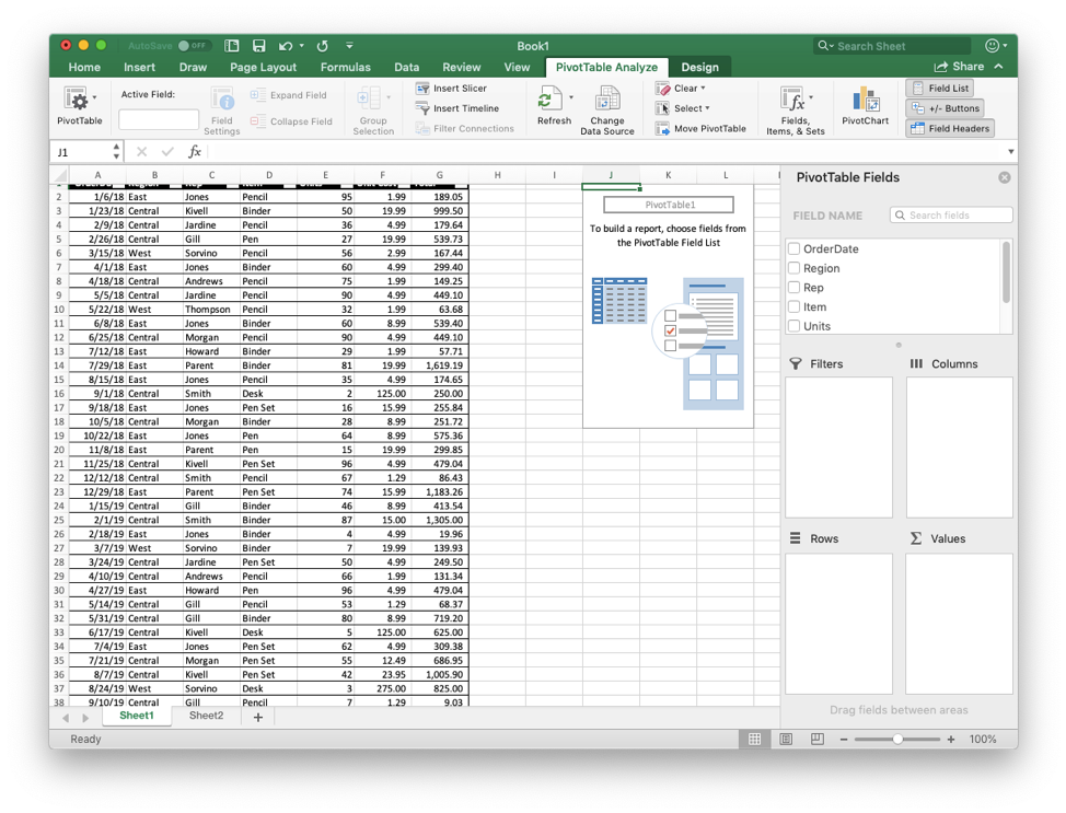
- Now choose the fields that you want to add the report. We selected Region and Rep from our example.
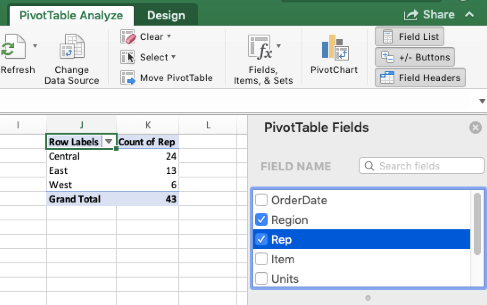
- Finally, we want to rename “Row Labels” in J1 to “Region”
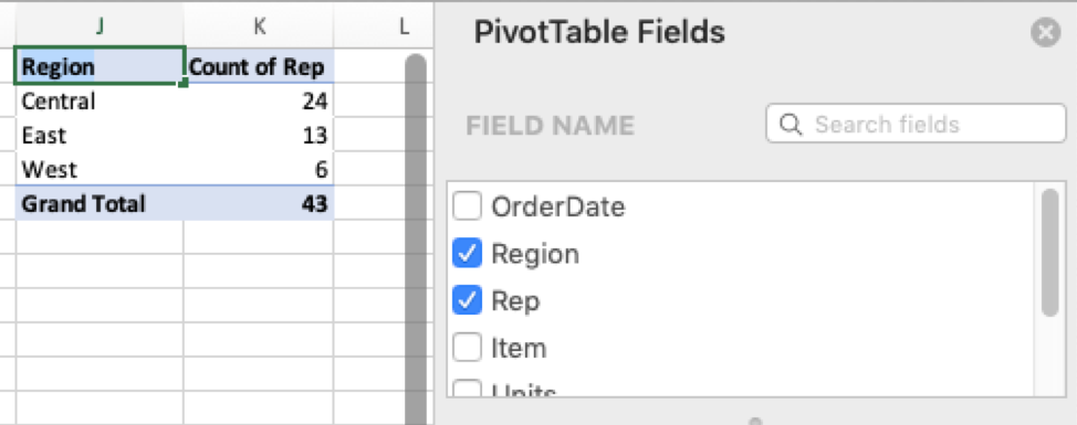
There you go! By following these steps, you have created your first Pivot Table. If you want to make a separate report in spreadsheet, instead of selecting a cell on the same Sheet, you can create a new sheet, select a cell and go from there.
If your organization uses Excel for reports, we offer private group Excel training. Contact us for more details.